A Nagging Question
“How long does it take to win a game of Bingo?” That’s the thought I had as I was calling my 20th Bingo game at my annual family reunion. “The game has to have an average length, right? It definitely feels like it,” I thought as I briskly roll the cage, filling the domed plastic sheet with each ball. “But how could I calculate that..?” After getting home, I got to work finding the solution. This is is an exploration into my process.
The Game
To answer any question about a game, we need to elaborate on its structure and rules. In Bingo, every player has a card with a 5x5 grid. They have the goal of creating a pattern on the grid by marking squares. The standard winning patterns are:
- any row of 5,
- any column of 5,
- or either diagonal of 5.
The center of the grid is considered “free,” such that ever player starts with that square marked. Every square besides the center is given a random number 1 thru 75 such that no number will show up on a card more than once.
The game is run by a caller who has a tumbler filled with balls numbered 1 thru 75. Each round, the caller randomly pulls a ball from the tumbler and announces it to the players. If a player has the corresponding number on their card, the square with that number is marked. The ball removed by the caller is not returned to the tumbler. This continues until a player’s card meets one of the winning condition and yells the titular "Bingo!"
So… how long does it take for at least one player to meet a winning condition?
My Shame
Unfortunately, I’m not a mathematician by education. Worse, I’m a former physicist turned businessman with a spreadsheet: something akin to a chimp with a machine gun. I know statistics, and a part of me feels like this can be done strictly on paper, but such a solution is not clear to me. Given that, my first route was to simulate the solution. I’ll be using Python to create the simulation and the graphs that follow; the full code be viewed at this link. Please be kind.
Permutations
It’s tempting to start by simulating the tumbler with generating a random number 1 thru 75. However, this isn’t accurate. If we do this, there will be a chance that the same number will be chosen twice. That would simulate the caller pulling a ball from the tumbler then placing it back inside. We want to simulate the caller pulling a number without replacement. In mathematics, this can be represented by a permutation. We will start with all numbers 1 thru 75 and shuffle them. This effectively generates the entire game’s pulls all at once for the simulation to run through.
We can use this same method to generate our player’s card by making a new permutation and choosing the first 24 numbers to populate our array. Using a permutation like this guarentees that the card will not have repeating numbers. (In a real Bingo game, each column labeled with each letter of the word “Bingo” can only be of sets of 15 numbers. For example, the column “B” will only ever have five numbers from the set 1 to 15, column “I” only from the set 16 to 30, and so on to "O". While we could simulate this strictly, the answer would not materially change.)
Mapping a Board States
A Bingo card encodes two sets of values:
- the array of numbers held in the grid that the player sees,
- and whether or not the squares of the grid have been marked.
I chose to create this mapping with two arrays, one which passes information to the other. The first array will hold the Bingo card’s numbers. The second array would hold binary values, 0 or 1, for a square that is either not filled or filled, respectively. The secondary array will start with all zeros, except for the center which will be initialized to 1 to represent the free square. If a number is called and it appears on a players card, our program will note the coordinates in our first array and mark that same coordinates in the second array with a 1. This may not be the most efficient way to create this mapping, but it makes intuitive sense for me. I hope it does for you too.
Winning
Now, we’ll quickly throw together a way to check our second array to see if, after each call, a card has won. Looking ahead, we plan on doing hundreds or thousands of simulations. To save just a little processing time, the code will check first that the sum of the marked array is greater than 4. This will make sure the code doesn’t run through all of the win conditions for a card that couldn’t possibly win, since you need a minimum of 5 squares to be filled for a win.
The Loneliest Number
Now, we can run our simulation. We will start simply and see how many pulls it takes for a single card to win. But, running it once...doesn’t help much. The number of turns to win will always be different! Instead, let’s run this simulation a few... thousand times and keep track of how many turns it takes for our single player to win. The Law of Large Numbers says “the average of the results obtained from a large number of independent random samples converges to the true value, if it exists.” Running this program over and over again, we can create a relative frequency histogram to visualize this convergent trend. The x-axis shows how many rounds it took any game to end. Once a game ends on that value, it increases the y-value of that bar by one.
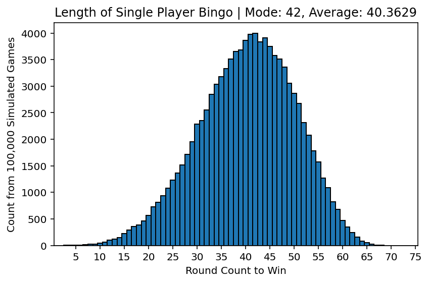
Frequency analysis like this is an entire topic of its own, but we can quickly say two things about this distribution. The mode of this distribution--the x-value that appears the most--is 42. So, a single player is most likely to play 42 rounds before they meet a winning condition. The average is slightly lower at around 40.3. While it is tempting to use the mode of the distribution, the nature of our randomly generated simulation will cause it to vary quite a bit at lower simulation counts, so we’ll consider the average moving forward.
Let's Make Some Friends
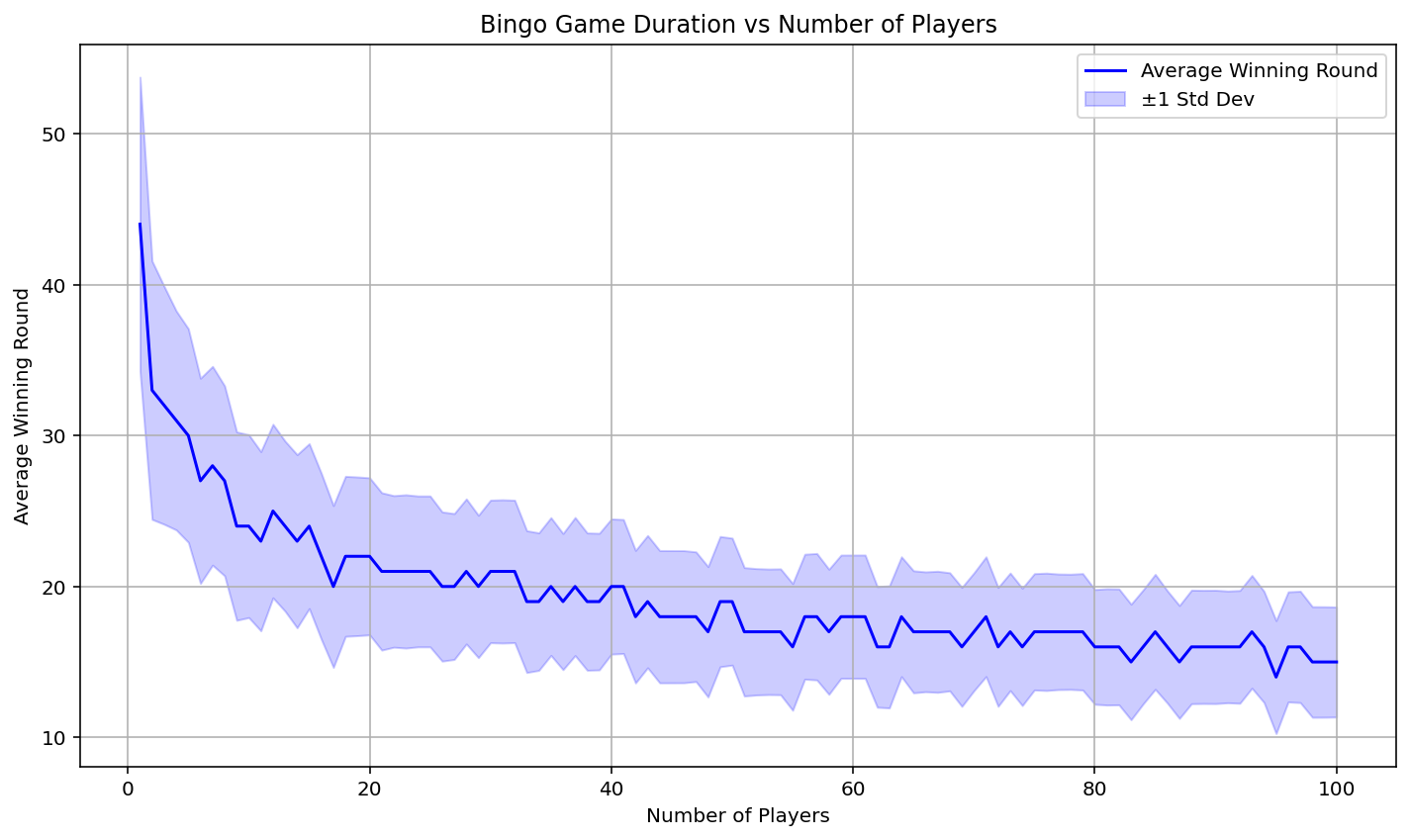
I can’t imagine a lot of people play Bingo by themselves. We’ve shown that it can be simulated in a completely probabilistic way, so playing solo would be the equivalent of flipping a coin over and over by yourself. An interesting question may be: how does the average game length change as we increase the number of players? After all, at my family reunion, we had various numbers of players at different times. We can run multiple simulations with different numbers of player cards and plot each scenarios’ average as a point along a segmented line. For this, I ran each scenario 7,000 times. This will cause our average to vary more at each simulation, but it will also lower the run time. As we plot these points, a trend seems to form. The line graph created shows how when we increase players on the x-axis, the average number of turns decreases on the y-axis.
Getting Fit
We could run this simulation for any arbitrary number of players, but the results above look like they might be following... a trend? Can we characterize what we are seeing here? This idea of creating a function to desribe our data is called finding the curve of best fit. If there is a function that our points follow, it will allows us to predict the average length of a Bingo game with any number of players without running the simulation and burning a hole in our CPU. Though, there are limitations to this concept, namely: our resulting equation will be continuous, but we’re modeling how the number of turns in a Bingo game varies with the number of players, both of which can only be positive integers. This is a good thing to remember when creating any best fit curve. Context always matters.
To start, we need to choose an equation that’s a contender to fit our data. Let’s see if we can make a few observations about our data to narrow down what that equation might be:
- The data decreases in y as x increases.
- The slope of the data is steep for small values of x, and the slope becomes flatter for larger values of x.
- It is possible that there is a vertical asymptote at x = 0. This can be explained as “a game with zero players will have an ‘infinite’ number of turns before there is a winner.”
- It is possible that there is a horizontal asymptote at y = 4; this can be explained as “a game with infinitely many players will have the shortest game of Bingo possible at 4 pulls. A win with four pulls will occur with any line that crosses through the free space at the center.”
Whenever I am looking for a trend, I like to look up pictures of families of functions. There are a few candidates that would satisfy our observations, but I’m going to try y=1/x. This equation does decrease in y as x increases, and it does fall off quickly before leveling out. It also has a vertical and horizontal asymptote. This feels like a good starting point.
With a candidate curve picked out, we want to generalize its equation to y = a/(x+b)^c+d. In this equation, b moves the curve left and right relative to the y-axis. We don’t need to do that, since there is currently a vertical asymptote at x = 0. So, we can set b to 0. Now, d will move our curve up and down relative to the x-axis. Since the standard curve has a horizontal asymptote at y = 0, we can set d = 4 to move our horizontal asymptote up to y = 4.
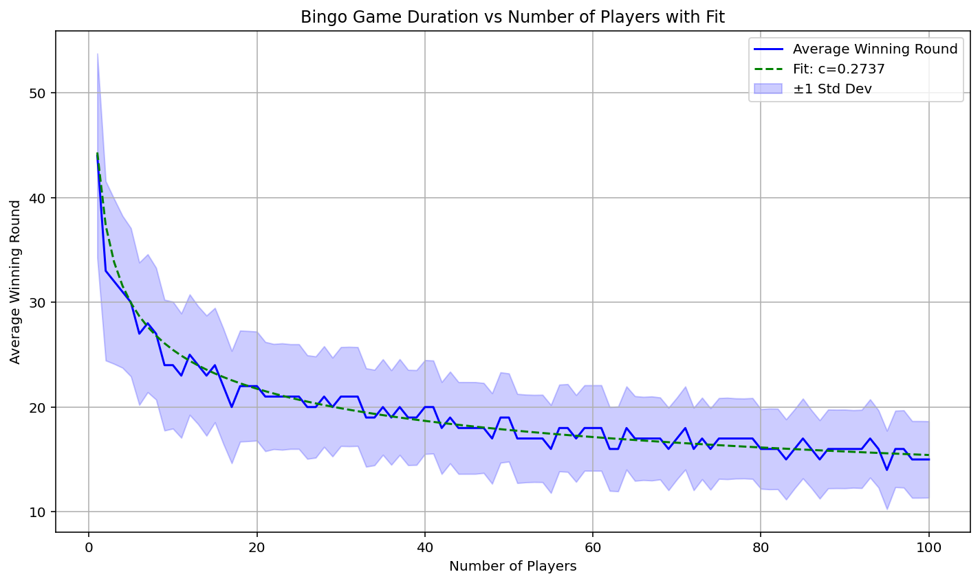
With only a and c remaining, let’s remember what x represents: the number of players in the game. We actually have a very good estimate for the average number of turns for a single player! It’s our average from earlier: 40.3. Let's plug in x = 1 and y = 40.3 to get: 40.3 = a/1^c. We know that 1 to any power c will always be 1, so a = 40.3. The only variable remaining is c. We’ve run out of clever tricks, so this last variable will need to be found using a curve fitting function in Python which hunts for an optimal value with brute force.
Results and Conclusion
Et viola, we get a really good fit! The average number of rounds of a standard game of Bingo can be described as:
y = 40.3/x^0.2737 + 4 where x and y are positive integers.
And with this function, we can give the average count of any Bingo game. Say that I know there will be ten people playing Bingo at my next family reunion. I can input x = 10 and find that, on average, each game will be about 25 rounds long! More analysis of Bingo can be done from here. One paper that I found by a student(?) at Berkeley named William Chon actually went one step further to calculate the number of near-miss games and went on to investigate the implications for those near-misses on running Bingo games at casinos. I would recommend giving it a read.
So, that’s it. We found a satisfying answer to our question. Starting by understanding our game, creating a set of rules. Then, we created a simulation that ran though games of various player counts. Using this data, we found a candidate best fit curve function to describe the data and used our fundamental understanding of the game to reduce the number of variables we needed to find.
If this has gotten you interested in learning more about this kind of approach, MIT Opencourseware has a good set of lectures describing simulations using random variables.
Thanks for reading!